Saikat Kumar Dey - A Simplified Implementation of Quicksort

Quicksort is a beautiful algorithm. It’s considered the fastest sorting algorithm in practice. Most implementations I’ve seen online are complicated. This post will demonstrate a simple implementation that trades space complexity for readability.

How does quicksort work?

3 steps.

Choose a pivot element.
Partition: Put all elements smaller than the pivot in a smaller array, (say, smaller_subarray). Put all elements greater than the pivot in another array (say, greater_subarray).
Recurse & Merge: Recursively sort the smaller and greater sub-arrays. Merge the sorted arrays with the pivot.

How do we implement it in Python?

Let’s start with the high-level function quicksort()


def quicksort(array: List[int]) -> List[int]:
    """Recursive implementation of quicksort.

    Args:
        array (List[int]): a list of integers

    Returns:
        List[int]: sorted array
    """

    # Base case
    if len(array) <= 1:
        return array

    # Step 1: choose a pivot
    pivot_idx = random.choice(range(len(array)))

    # Step 2: partition
    smaller_subarray, greater_subarray = partition(array, pivot_idx)

    # Step 3: Recurse on smaller and greater subarrays.
    return (
        quicksort(smaller_subarray)
        + [array[pivot_idx]]
        + quicksort(greater_subarray)
    )

Let’s go line by line,

Base case

 if len(array) <= 1:
     return array

Every recursive function must have one. If we have an empty or single-item array, there’s nothing to sort. We simply return the array.

Step 1: Choose a pivot

pivot_idx = random.choice(range(len(array)))

The choice of pivot is the difference between having an O(N log N) vs O(N^2) time complexity.

How so? Let’s take an example.

The worst-case involves having an already sorted array.

array = [1,2,3,4,5]

The image below shows recursion trees using two different pivot selection strategies:

Legend

Blue lines => the greater subarray.
Orange lines => the smaller subarray.
Red lines => the pivot.

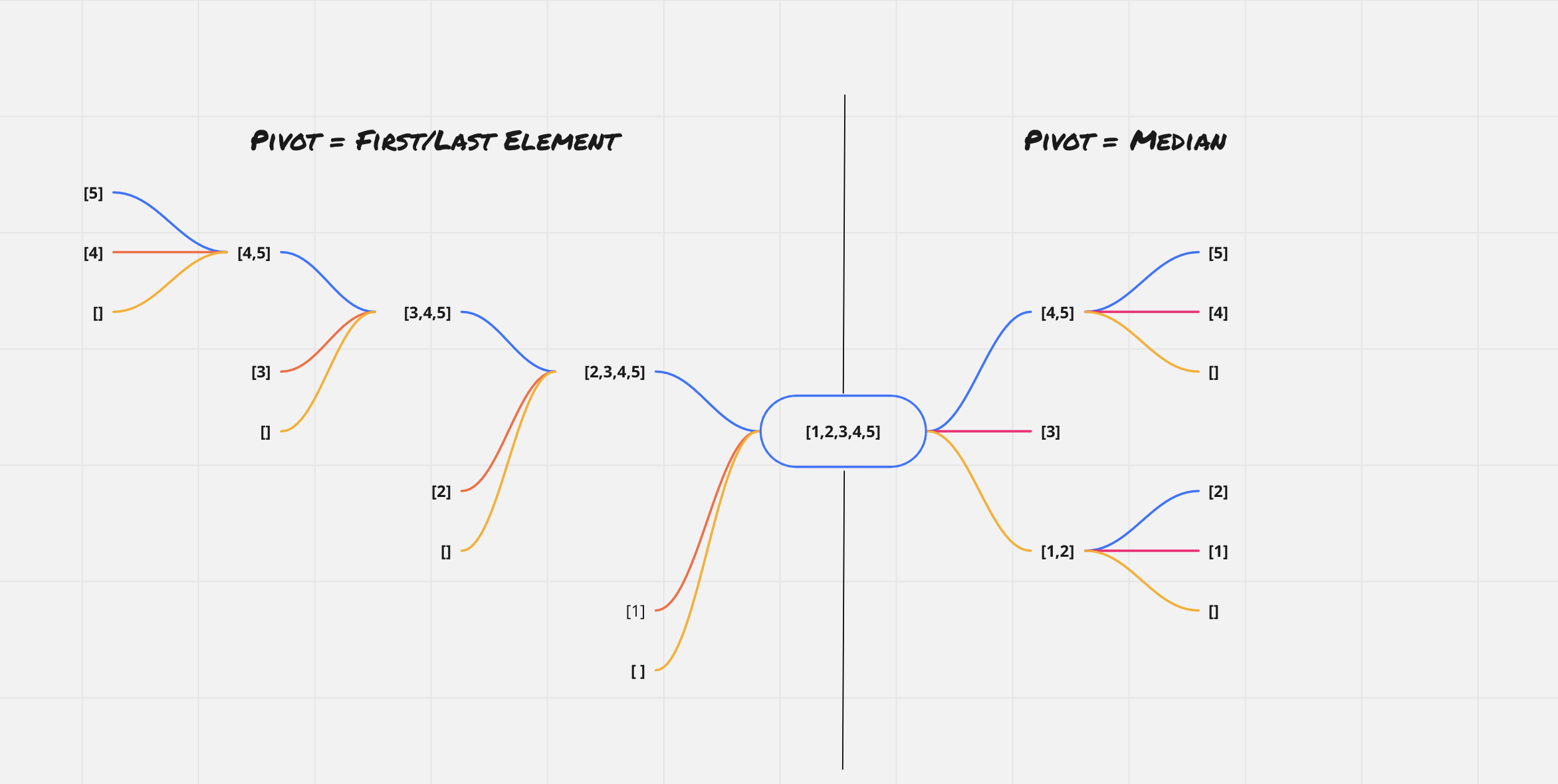
Left shows the case where we always choose the first/last item as the pivot. This leads to higher recursion depth as the subproblem size reduces by 1 at each level. We have roughly O(N) levels / recursive calls. Since joining the sub-arrays with the pivot is O(N), this leads to O(N^2) time complexity.
Right shows the ideal case where we choose the median as the pivot at every level. This leads to balanced sub-problems. The recursion depth is lower, roughly O(log N). This leads to O(N log N) time complexity.

Choosing a random pivot leads to an expected runtime of O(N log N) time complexity. We use that in this implementation.

Wait! There’s still one case where quicksort() could be O(N^2), even after choosing a randomized/median pivot. This is the case when every item in the array is identical. We could add a check to avoid this case as well.

According to this source ,

The probability that quicksort will use a quadratic number of compares when sorting a large array on your computer is much less than the probability that your computer will be struck by lightning!

Step 2: Partition

We write the high-level function assuming that we have a magic function partition() which returns two arrays.

smaller_subarray: all elements <= the pivot
greater_subarray: all elements > the pivot

The implementation of partition() is quite simple. We compare each item in the array with the pivot. If it’s <= pivot, we add it to the smaller sub-array, else we add it to the greater sub-array.

def partition(array: List[int], pivot_idx: int) -> Tuple[List[int], List[int]]:
    """Parition array into subarrays smaller and greater than the pivot.

    Args:
        array (List[int]): input array
        pivot_idx (int): index of the pivot

    Returns:
        Tuple[List[int], List[int]]: smaller subarray, greater subarray
    """
    smaller_subarray, greater_subarray = [], []
    for idx, item in enumerate(array):
        # we don't want to add pivot to any of the sub-arrays
        if idx == pivot_idx:
            continue
        if item <= array[pivot_idx]:
            smaller_subarray.append(item)
        else:
            greater_subarray.append(item)
    return smaller_subarray, greater_subarray

Step 3: Merge

return (
        quicksort(smaller_subarray)
        + [array[pivot_idx]]
        + quicksort(greater_subarray)
    )

This step is quite exquisite. We recurse on the smaller and greater sub-arrays and place the pivot in between them. The beauty of a recursive implementation is that we could re-use our function with a smaller size of the input and trust that it would work.

Let’s unroll it a bit.

quicksort(smaller_subarray) => returns a sorted version of the smaller_subarray
[array[pivot_idx]] => out pivot in a list. It’s needed for concatenating it with the other two lists.
quicksort(greater_subarray) => returns a sorted version of the greater_subarray

Now, we join the 3 lists including the pivot, and return the final sorted list.

Complexity

Time

Expected run-time of O(N log N) since it’s a randomized implementation.

We do O(N) work at each quicksort() call. The major components are partition() and merge step - both are O(N).

For randomized implementation, we have O(log N) levels/recursive calls.

So, expected time complexity ~ Number of recursive calls * work done per recursive call ~ O(N) * O(log N) ~ O(N log N)

Space

O(N) since we use extra space for storing the smaller and greater sub-arrays. The recursion stack also uses O(log N) space. Overall, this implementation uses O(N) space.

The in-place implementation without using auxiliary lists would lead to an O(log N) space complexity.

The code

The implementation including the partition() and tests are here.